Chapter 4
Spirals of Many Shapes
We must admit to you reader that nearly everything beyond this point is our humble attempt to explain this masterpiece of a Stack Exchange post. We’ve played around with circular and elliptical tracks, but what about star shaped tracks? Flower shaped tracks?? 3D tracks??? Let’s try and generalize our equations to work with any track! Throughout our journey, we’ll be applying what we find for an elliptical track as an example.
For this chapter, we’re going to be using a lot of the lessons from previous chapters, like parametrics, arc length, and offset. By the end of this though, you will be a spirograph and trochoid master!
Defining our track
In Chapter 3, we rewrote our hypotrochoid equation so that we could define the ellipse as a parametric equation. Using that idea, this chapter will also define our track as a parametric equation, but will keep it general so we can use any track!
To review, for an ellipse:
Rotation of the Tracing Wheel
Finding the Arc Length of the Track
In Chapter 1, we saw that the rotation of the tracing wheel is determined by the distance travelled along the track:
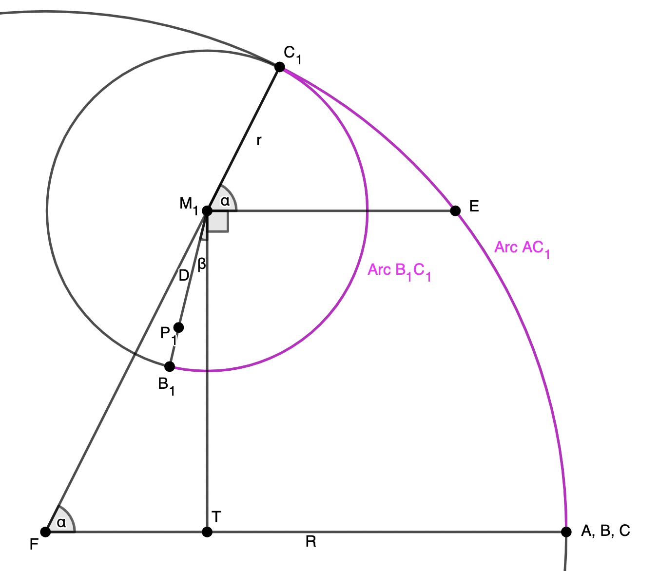
So in this diagram of a hypotrochoid,
Where does this equation come from?
From calculus’ greatest friend: approximation with refinement. We can approximate a parametric curve as a bunch of tiny
little lines. Take a look here.
Applying this equation for an ellipse, we can find that the arc length for a given
Representing our Tracing Wheel as Parametrics
I know, I know, it’s parametrics all around, but we need a way of turning this distance into some rotation. Since we’re already in parametric land, it makes sense to also define our tracing wheel as a parametric.
What is this notation?
Dealing with rotations and other transformations can get complicated (and we’ll be doing a lot of that in the next section).
Since this only has one column, it’s exactly the same
Here,
But if we’re tracing our spirograph counter-clockwise, then the tracing wheel will spin clockwise (remember it’s rolling!). So, let’s change the direction of our parametric equation by making
It’d be nice if we could define our parametric so bottom-most point on the circle is at the origin. This way, we don’t have to worry about offsetting the wheel later like we did in Chpater 3.
Let’s see what we got so far!
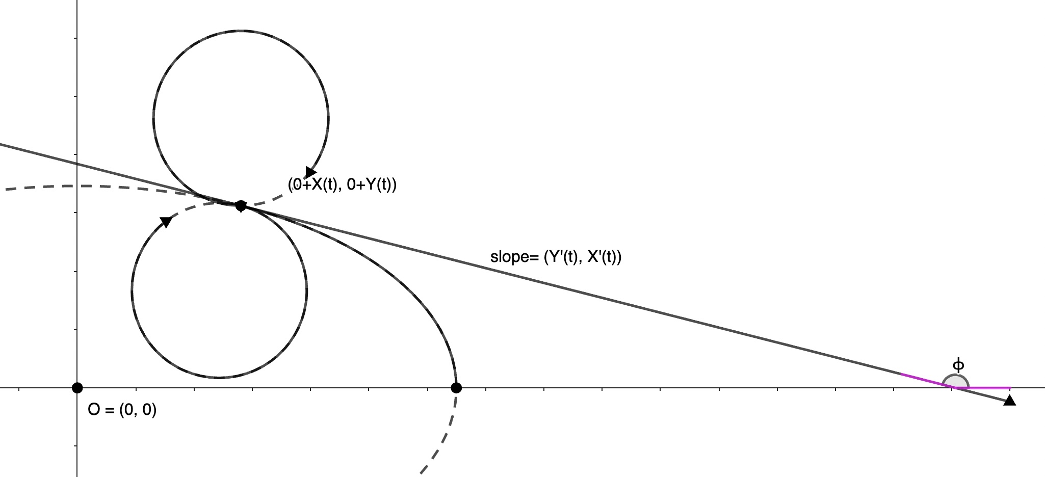
Let’s also redefine where we are at time u=0 to the origin! This way, it’ll be easy to attatch this to the point of tangency. To do so, we find the angle (let’s call it
Now, let’s modify our equation now with this angle!
We haven’t yet accounted for the position of the pen point. Replacing
Let’s see what this like!
Find that Rotation!
Now, let’s roll the circle!
Remember, rolling without slipping requires that the distance travelled around the track equals the amount of the wheel rolled. The arclength of our circle parametric is
Substituting this in, we get the final term representing the rotation of the tracing circle!
Position of the Tracing Wheel
But we’re not done yet! This is what we have right now:
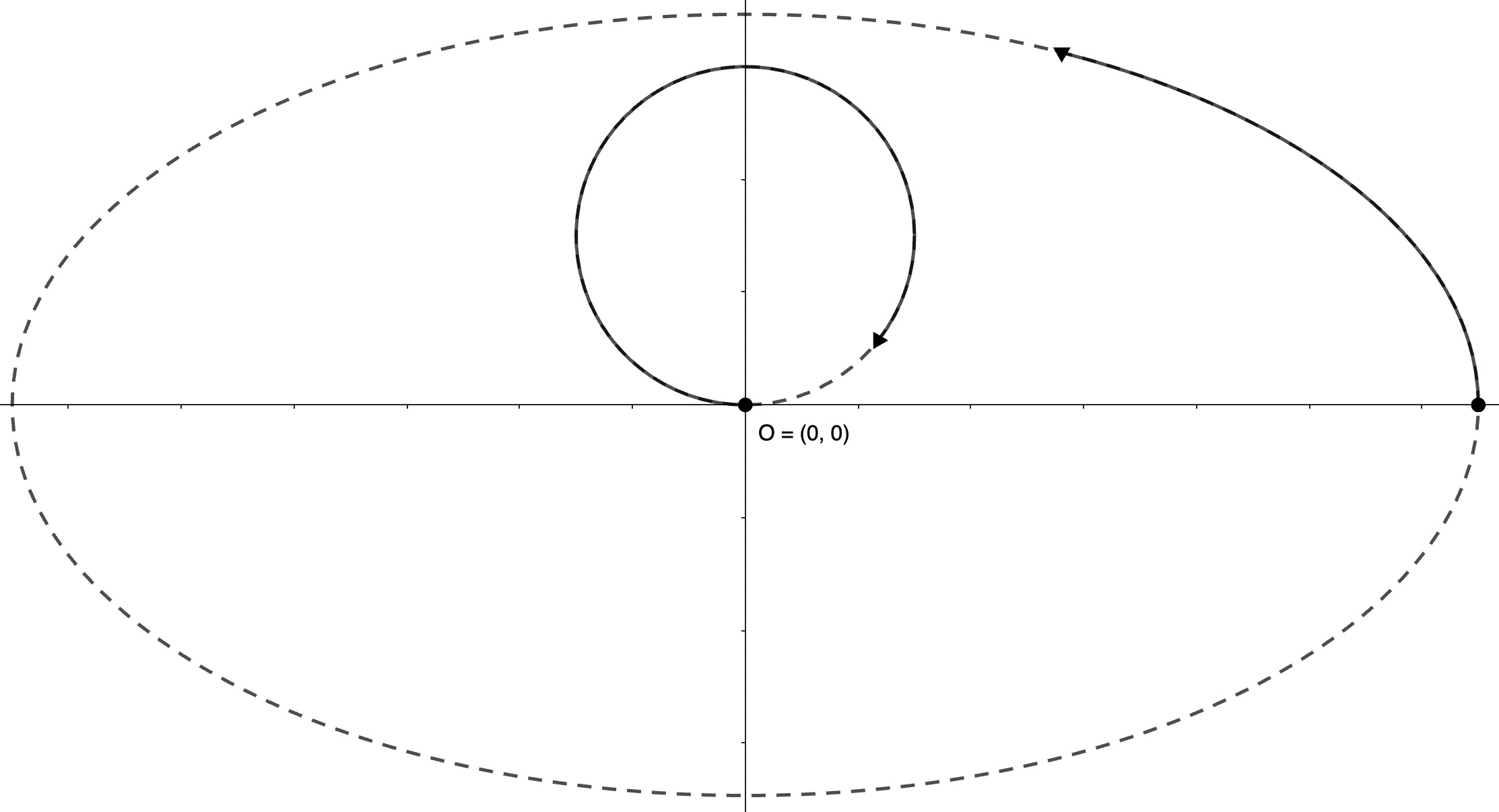
(Where those two black arrows are the same length).
We have to account for the position of our wheel and make sure that the point where the parametric equation for the inside wheel begins (it’s at the origin right now) aligns to the point where the equation for our track begins!
For this, we need to do two more things: translate our tracing circle so that it touches the ellipse, and then rotate our tracing wheel so that it rolls properly.
Translating our Circle
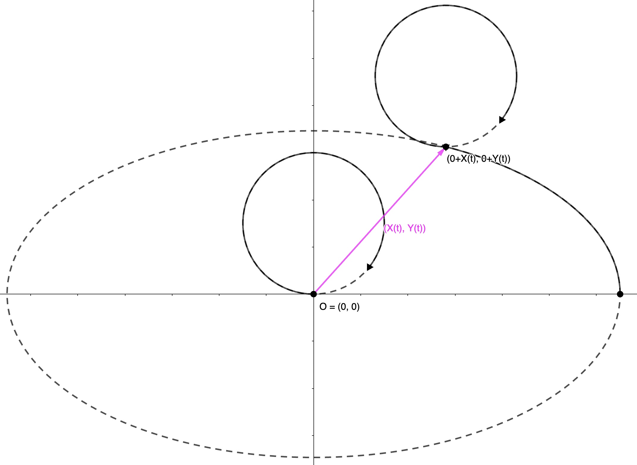
To start, let’s move our tracing circle to the point on the track. As we saw in Chapter 3, we can just add the parametric of the track to our equation:
Doing this gets us:
Rotating Our Circle
Next, let’s rotate our circle so that the parametric equation where our circle begins
To do so, we need to rotate by some tangential angle
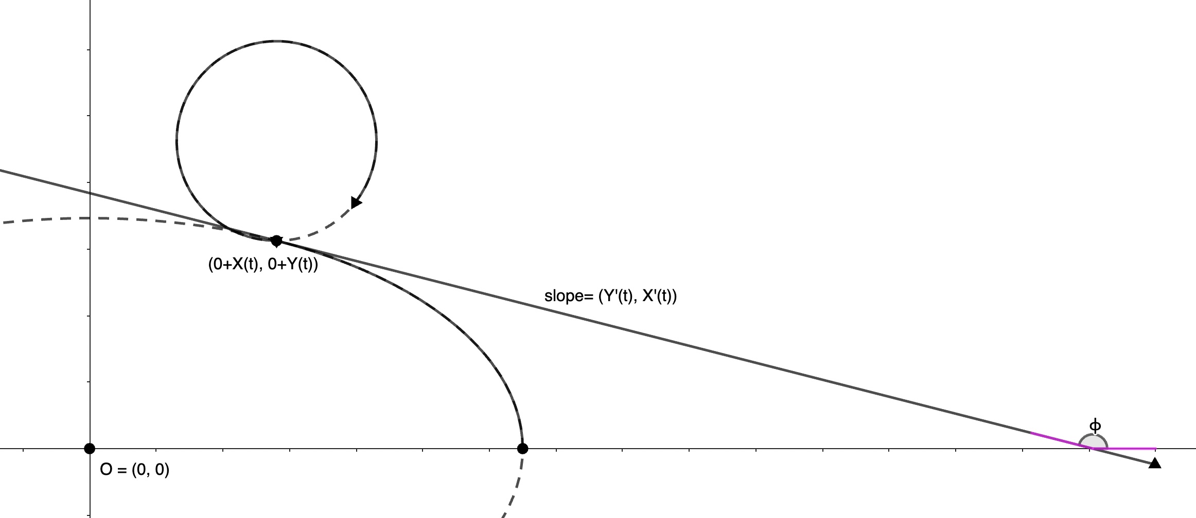
To have the wheel roll inside the right way inside the track, we should rotate it anticlockwise into the right position. To do this, we can plug in
And you can see, after doing this rotation:
It looks pretty good!
Since we’re in the land of linear algebra, all we need to do to apply this rotation is to multiply it by the parametric of our tracing circle! (It’s important we do this before our translation though!)
And there we go! That’s our final equation!!
Playing Around
Ding, Dong, it’s a Desmos Song!
(As you can see, the major down-side here is that it’s not the easiest to simulate). That was a lot of math, but hopefully now you are ready to make some crazy spirals! Here are some challenges you can explore further too!
- A wheel moving along a graph?
- A wheel moving inside of a star?
- A wheel moving inside of a wheel inside of a fixed track?
- Different shaped tracing shapes?
The world is your track, go make some spirals!