Chapter 3
Around an Elliptical World
Be warned fellow traveller. In this chapter, we venture outside the world of the spirograph into that mysterious and frequently terrifying world of theory. First, we will explore a way of apporximating the path traced by a spirograph with an elliptical track. But in the next chapter, we will not only make this approximation exact, we can generalize our equations to make a spirograph with any track imaginable.
For our first method, instead of starting from scratch, let’s break down the equations we got for a circular hypotrochoid from Chapter 1. We can then edit them to describe an elliptical track.
Let’s rewrite this out so we have three terms:
The first term of both equations describe the track: a circle with a radius of
Now, to start replacing these terms to describe our elliptical track. But to describe this track, we must first ask:
What Is an Ellipse?
For our purposes, an ellipse is just a squashed circle. Being a squashed circle, it no longer has 1 radius, but needs to be described with the biggest radius and the smallest radius, called the semimajor and semiminor axes respectively.
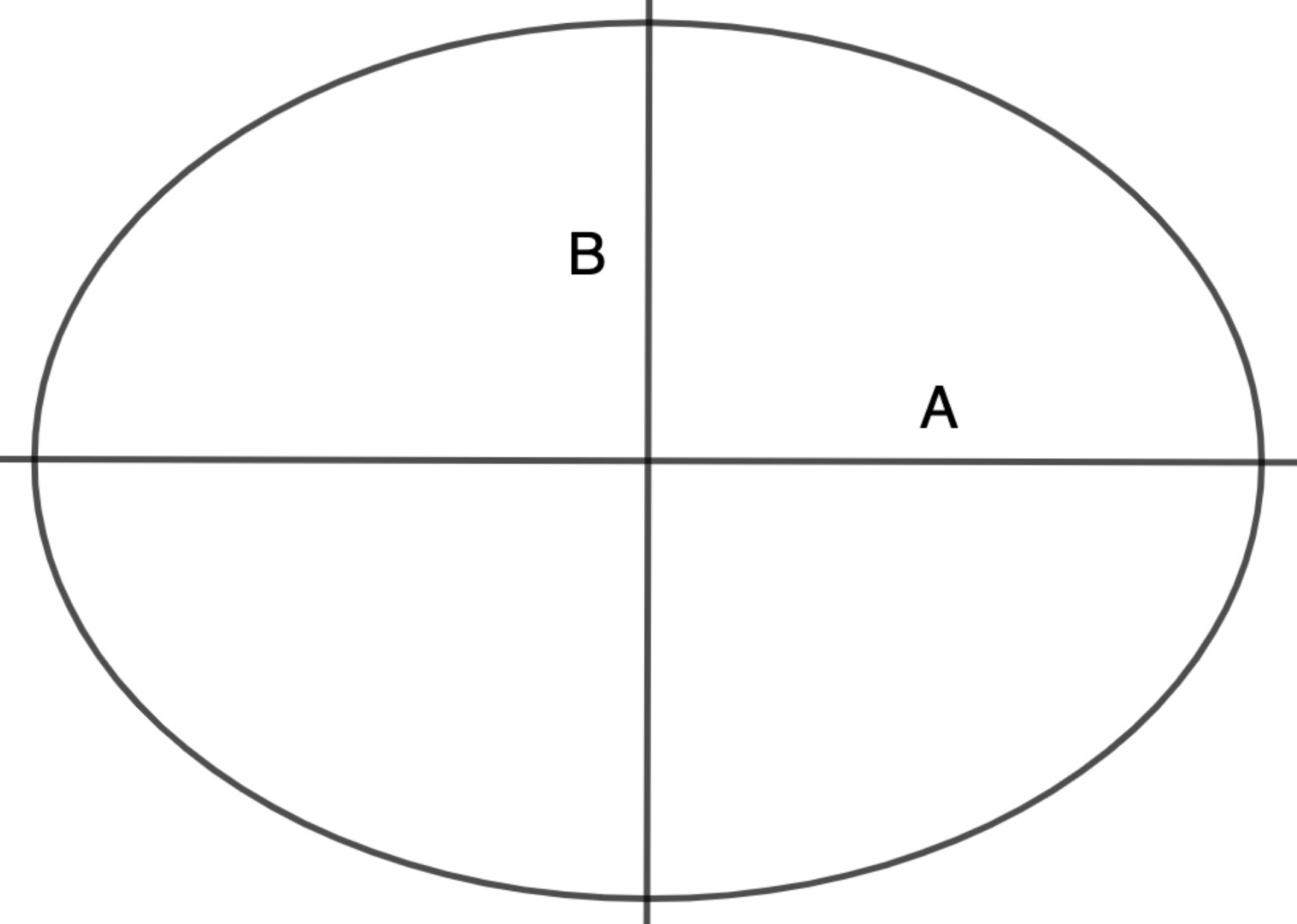
Let the semimajor axis have a length of
Wait, why a
Notice how we’re making the distinction between
Replacing this parametric in for our first term gets us:
A Saving Approximation
Second problem: we’ve replaced the
That idea still holds true since we’re still rolling the tracing wheel! Calculating the exact length of that arc for an ellipse gets more complicated, so for now we can introduce an approximation. We might not know the exact arc length of the ellipse, but we can know the perimeter of the ellipse:
Finding the radius of a circle with this perimeter will give us a good enough approximation for
Perimeter of an ellipse side tangent
What we show above is known as the elliptic integral, and it gives off the accurate value for the perimeter. It’s
derived from finding the length of the parametric curve, which we discuss a little in the next chapter. The elliptic
integral is famous because it can’t be written in elementary functions,
but that hasn’t stopped mathematicians from trying!
Finding Our Center
We’ve done so much math but we haven’t had a single Desmos for this chapter. Let’s fix that and graph what we have!
Hey! That looks pretty good! Wait, what is that?!
What’s what?
Try making the track super squished by making
Answer
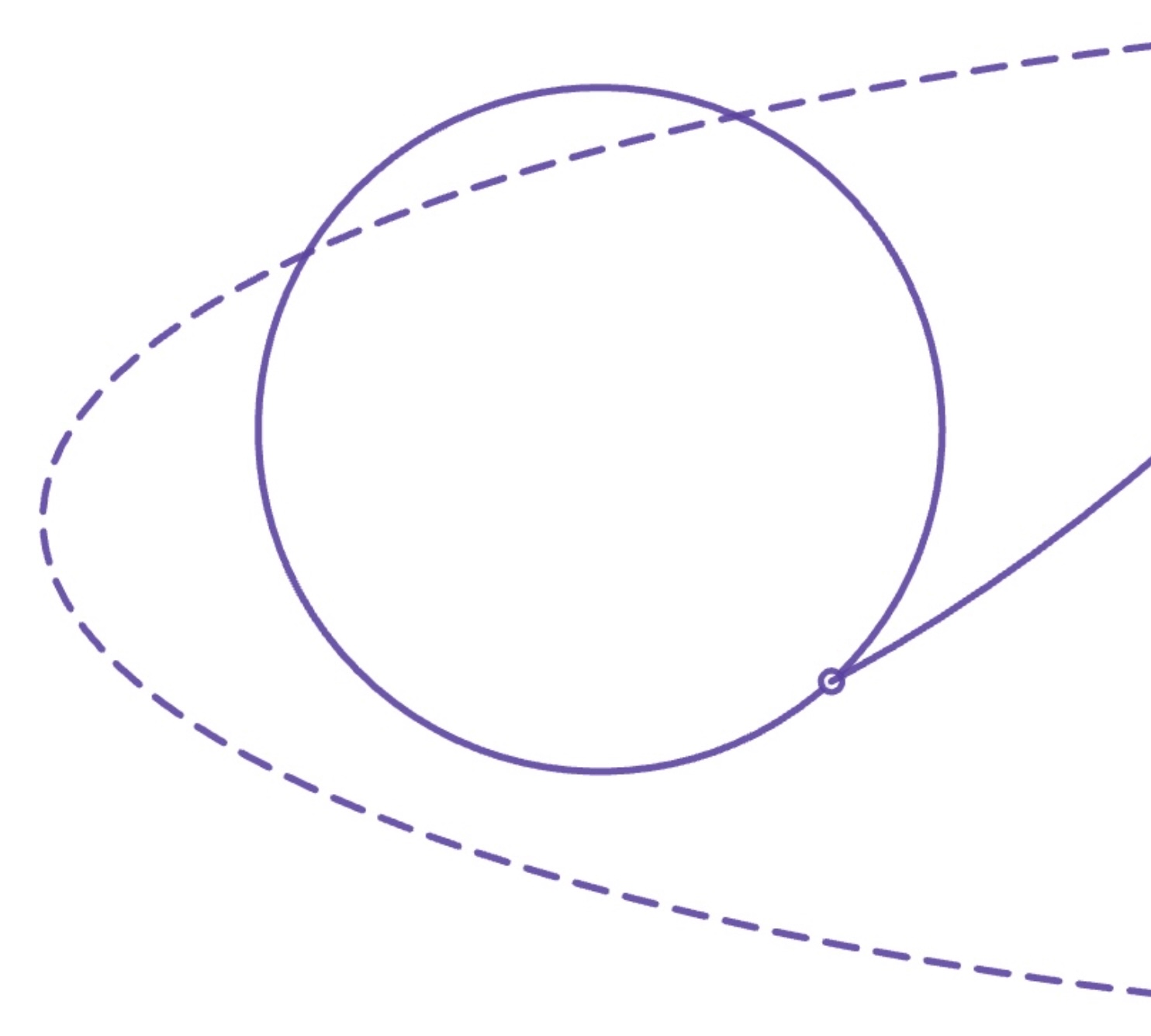
The rotating circle is clipping through the track!
The problem is that we still haven’t edited that second term, meaning the center of our rotating wheel isn’t correct. Let’s look at a diagram from Chapter 1 when we were working with a circular track:
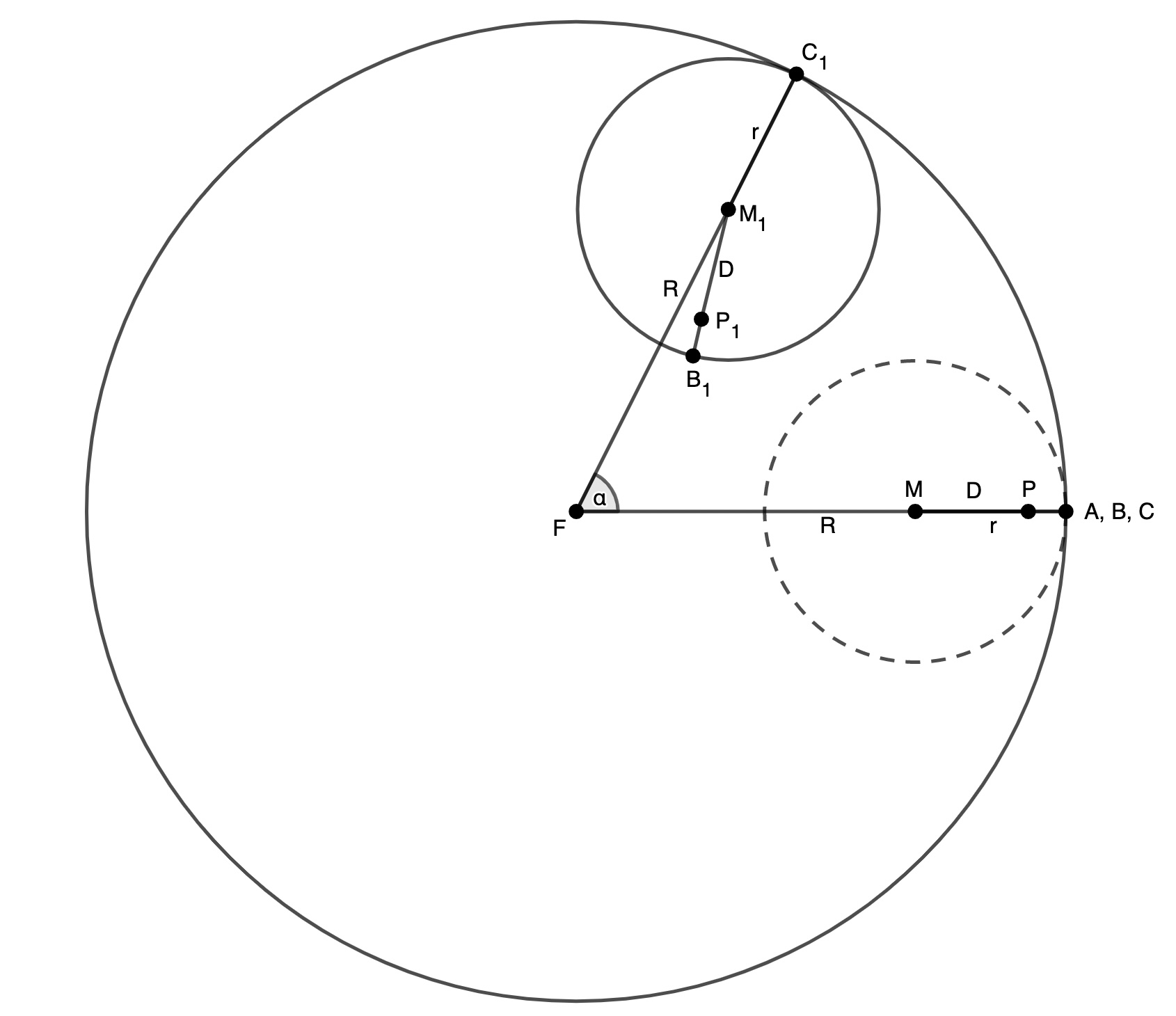
Notice how the point of tangency (point
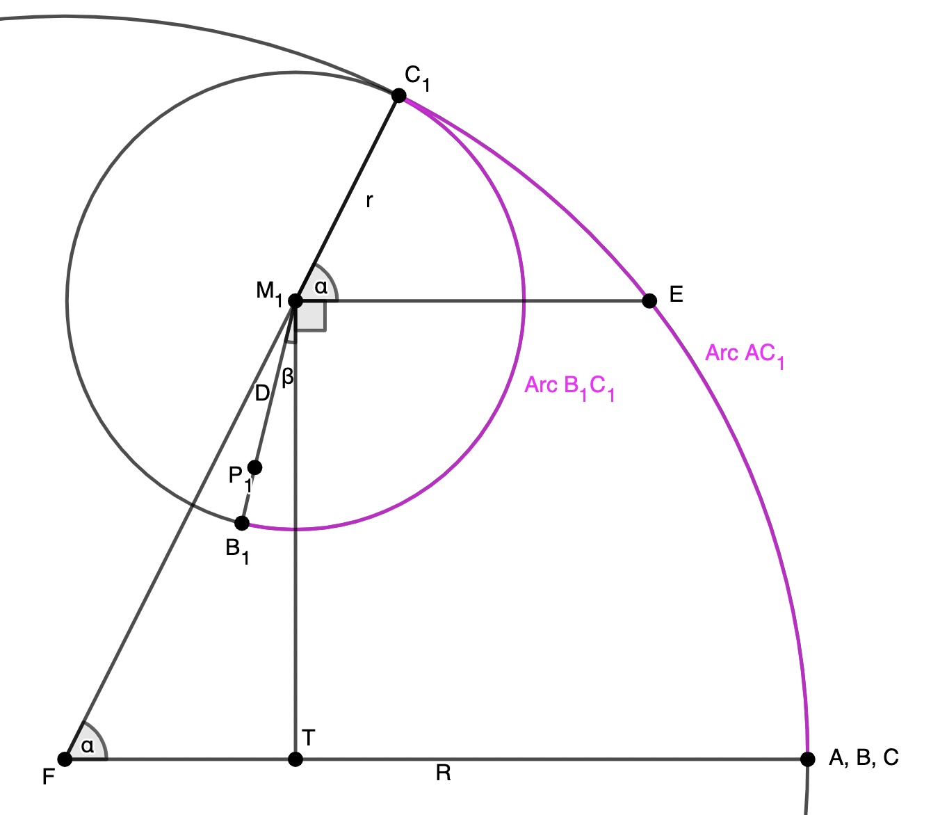
Compare this with a diagram of an elliptical track:
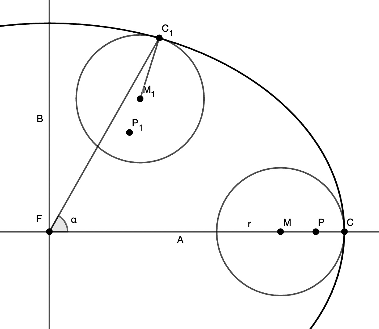
The point of tangency and the two centers are no longer collinear, so the equation
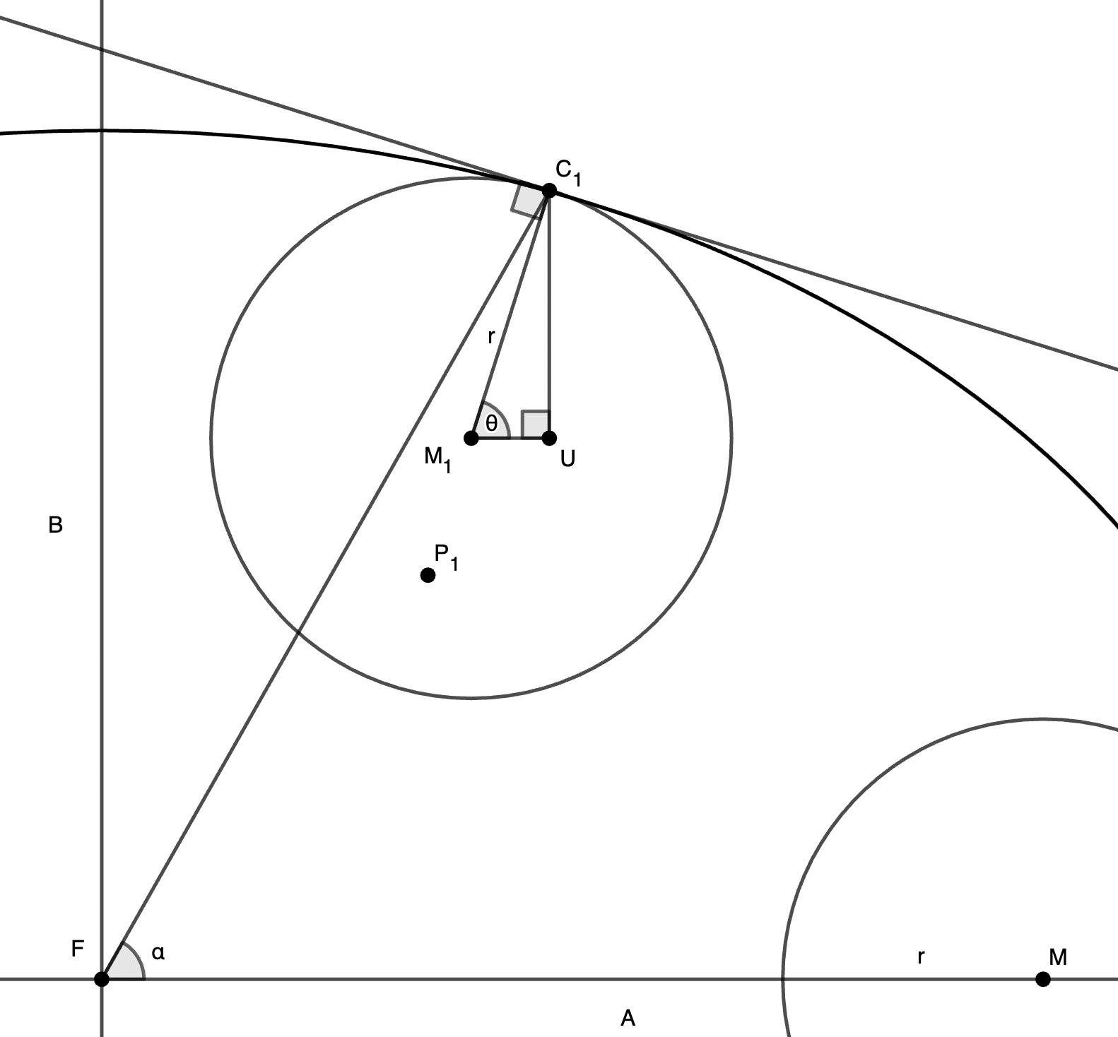
To find this slope, (equal to
All we need to find now is the lengths of segments
Awesome! All that’s left to do is to replace our offset terms with these and we’re good to roll!
(don’t those equations just look lovely)
Playing Around
What’s that, is it Desmos-time?
Notice how the wheel kinda slips when it meets the pointer parts of the ellipse. This is because of that approximation we did earlier, but is something we can fix in the next chapter!